About
Notes on Professor Pedro Domingos' 2015 popular science book
The Master Algorithm: How the Quest for the Ultimate Learning Machine Will Remake Our World (ISBN 9780141979243)
in which Domingos gives a fairly accessible account of the history of machine learning, from first algorithms to present day applications. Notably, Domingos builds a taxonomy of the major branches within the research community: the five "tribes" of machine learning.
This piece is a summary of the five tribes, with a little personal extra.
Thank you Eduardo for the book recommendation!
Sections marked with a star () contain supplementary material not mentioned in the book.
The Master Algorithm
Introduction
The purpose of machine learning is to have computers write their own programs. The real world is so complex, and desired software behaviour so subtle, that the human limits of explicit instruction programming are quickly reached. By instructing systems to learn from available data, the desired system behaviour can be synthesised much more quickly, accurately and efficiently.
The distinction between machine learning and artificial intelligence should therefore be clear: the broad discipline of AI is concerned with building capabilities that mimic human cognitive abilities, while machine learning is about the implementation of systems that learn from data. Learning is certainly a fundamental human faculty, so naturally machine learning has a place under the umbrella of AI.
The history of machine learning is a series of experiments in the design of learning systems. Research in this area has frequently been driven by specific applications, by mathematical discoveries, and by inspiration from the natural world. Many of the most capable systems today are variants or direct descendants of desceptively simple insights about the nature of learning. At the same time, different learners make different assumptions about learning from finite data, which makes them useful for certain things, but not for others.
Pedro Domingos argues in his book that as present day machine learning algorithms generally do well in a number of disparate application areas, perhaps a more general purpose learning system could be within reach. What if one learner could do everything, could learn all there is to learn from data?
The Master Algorithm Hypothesis:
All knowledge — past, present, and future — can be derived from data by a single, universal learning algorithm.
The Master Algorithm is a call to arms for a grand unification effort, the quest for the Master Algorithm, the ultimate learning system. Instead of working in isolation from one another, the major schools of thought — the "tribes" — of machine learning would do well to come together, for any Master Algorithm must be able to do it all.
Domingos' book is a whirlwind tour of machine learning, a review of the main methods and key principles around which the five tribes of machine learning have formed. Each tribe comes with its own colourful characters and horrible histories. Domingos is an enthusiastic narrator: in addition to the technical subject matter, the book is full of real-world applications, biographical snippets and all kinds of intrigue and drama.
Domingos' draws from his long academic career and paints an insightful picture about the state of machine learning today and how the field ended up where it is. Domingos' storytelling builds up to a concrete proposal for the ultimate learning machine, a blueprint for the Master Algorithm.
And it turns out that the work to realise it has already begun.
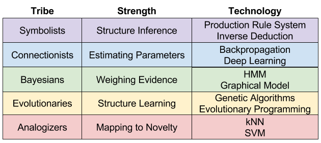
The Five Tribes
- The Symbolists
- The Connectionists
- The Evolutionaries
- The Bayesians
- The Analogizers
Domingos describes the tribes like so: "Each tribe has a set of core beliefs, and a particular problem it cares about the most. It has found a solution [..] and it has a master algorithm that embodies it."
The Master Algorithm is a journey across the territory of each tribe.
Machine Learning Lingo
- Rationalist/Empiricist
- Rationalists believe that senses deceive and that logical reasoning is the surest path to knowledge. Empiricists believe that all reasoning is fallible and that all knowledge must come from observation and experimentation.
- Generalisation — Hume's problem of induction
- Looking at data with contradicting patterns, *you have no basis to pick one generalisation over another*. You must *assume* that future is like the past, or knowledge in general is impossible. And there's more: this principle only works for exact experiential matches: reality is tricky because of novelty.
- Newton's principle
- "What is true of everything we've seen is true of everything in the universe."
- No free lunch
-
Pick a learner that is accurate for unseen data. There exist worlds in which all the labels of the unseen are flipped. Because of (tailored) pathological cases, all learners are equivalent to coin flipping.
Fortunately we primarily care about worlds that agree with reality: again, we must assume things, or knowledge is impossible. These assumptions are found under the rubric of bias in machine learning. The quest is about finding a useful learning machine that can learn everything from the simplest set of assumptions.
- Bias and variance
- If you keep making the same mistakes, the issue with your model is *bias*, and you need a more flexible learner. If there's no pattern to the mistakes made, the issue is *variance*, you can try making the learner less flexible. More data helps as well.
- Overfitting
-
For an unrestricted learner, two things are the same only if they are exactly the same. Learning is also about forgetting the irrelevant details, generalising to meet real-world variability.
A learner that does not generalise from data is overfitting. Overfitting occurs when there are too many hypotheses and not enough data to tell them apart — but there's a problem there as well.
Or as Domingos puts it: "A good learner is forever walking the narrow path between blindness and hallucination."
- The machine learning problem
- How do we generalise knowledge to situations that we haven't seen before?
- Combinatorial explosion
-
When the number of things an algorithm needs to do grows exponentially with the size of the input.
In some cases it's a double explosion, as inputs can grow exponentially as well. Fortunantely mchine learning methods can frequently eat away one of the exponentials.
- Noise
- Errors in the data, or random events that you cannot predict.
"It is possible to commit no mistakes and still lose. That is not weakness. That is life." — Captain Picard
- Dividing data
-
Overfitting can be tackled by dividing available data to a *training set* and a *test set*, where the former is used to build a model and the latter to verify its accuracy. There is a whole tradition and methodology around this process.
Statistical significance and can be used to further gain confidence in the learner's ability.
The Symbolists
For Symbolists, all intelligence is symbol manipulation. Questions can be posed as equations, and solved by replacing expressions with other expressions. Learning is built on pre-existing knowledge, and new problems are solved through a process of synthesis, where new knowledge is created through operations on existing knowledge.
The Symbolist master algorithm is inverse deduction, in which missing components that block a deductive resolution are identified and then made as general as possible. The related decision tree is a simple yet capable classifier that encodes knowledge as a series of choices.
Propositional logic
A proposition is a declarative sentence which is either true or false. Atomic sentences encapsulate knowledge and get marked with a symbol, typically upper case letters.
Sentences are combined by connectives:
- the conjunction ∧ (also &),
- the disjunction ∨,
- the implication ⇒ (also →, ⊃),
- the negation ¬ (also ∼),
- and equivalence ⇔ (also ↔, ≡).
For example, let:
- A = "Today is Tuesday"
- B = "Tomorrow is Wednesday"
- C = "Tomorrow is Friday"
We can encode statements, encapsulate knowledge about the world using this grammar:
- A ("Today is Tuesday", which is a [true] statement on Tuesdays)
- A ∧ B ("Today is Tuesday and tomorrow is Wednesday.")
- B ∨ C ("Tomorrow is Wednesday or tomorrow is Friday.")
- A ⇒ B ("If today is Tuesday, then tomorrow is Wednesday.")
- ¬C ("Tomorrow is not Friday.")
- A ⇔ B ("Today is Tuesday if and only if tomorrow is Friday",
also "If today is Tuesday, then tomorrow is Wednesday and if tomorrow is Wednesday, then todays is Tuesday.")
See any textbook on elementary logic for more.
Deduction and induction
Making use of logic in machine learning begins with the idea of identifying and extracting regularities captured by the available data.
Begin with a set of assumptions about data form, and check if you can answer your question through a series of logical operations — through symbol manipulation. If nothing fits the labelled data, relax the original assumptions, and try again with a more flexible form.
Logical reasoning is built on conjunctive forms (A and B), then on disjunctive forms (A or B), and finally on the most general forms, rules (A implies B, etc.). We can deduce new knowledge from atomic sentences but also build on previously established rules and sentences. This process is known as deduction.
Deduction:
Socrates is human.
All humans are mortal.
Therefore, _________
By deduction from the given statements, we can deduce that Socrates is mortal.
Induction, then, can be thought of as the inverse of deduction, in the same way subtraction is the inverse of addition.
Induction:
Socrates is human.
_________
Therefore, Socrates is mortal.
Specific inductive formulation to fill the gap:
If Socrates is human, then he is mortal.
But we have more data:
Plato is human. Plato is mortal.
Aristotle is human. Aristotle is mortal.
With Newton's principle:
If an entity is human, then it is mortal
Or,
Humans are mortal.
Decision trees
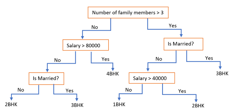
Deduction is computationally intensive. Decision trees help address situations where multiple rule sets match an instance. A decision tree solves the ambiguity problem through a game of "twenty questions".
Decision trees are classifiers. Each node of the tree asks a value of one attribute, and depending on the answer, we follow one or another branch. At the leaf, we read the predicted concept, a class. Each path from the root corresponds to a rule.
Decision trees can be learned with a divide and conquer approach: pick a test attribute, divide data by that attribute and repeat with a subset of data in each corresponding child node. When all data in a node shares a label, the node becomes a leaf with the label as the class.
Choosing the attribute to divide on is key: going for a low-entropy (high-similarity) subset is a good strategy. Satistical significance and weights help control for overfitting. With continuous data, key thresholds can be used to discretise the variable.
Decision trees are simple to implement and a great baseline. Decision trees are particularly interpretable, among machine learning systems.
However, sets of rules are exponentially more efficient at encoding concepts compared to decision trees. Generating a tree from a set of rules can blow up computationally.
Decision trees can also be used in an ensemble configuration, yielding a technique known as "random forests", or "random decision forests". The idea is to generate many decision trees in a stochastic process, and then select the most representative tree or the "average" tree for use in classification or regression. This process corrects for overfitting.
Knowledge engineering legacy
Symbolist machine learning is an offshoot of knowledge engineering school of AI, whose heyday was in the 1970s and 80s. Despite early promise, so called knowledge-based systems failed to deliver on AI hype, and the whole school effectively disbanded. Letting computers automatically learn from data proved much easier.
Knowledge acquisition bottleneck
Extracting knowledge from experts and encoding it as rules is too difficult, too labor-intensive, and too failure-prone to be viable for most problems.
The practice of knowledge engineering is still aligned with the Symbolists cause. Manually entered data is fed to Symbolists learners, including curated knowledge bases.
Contemporary applications
The Symbolists — Conclusion
The oldest tribe, with knowledge engineering and AI history. Symbolist school is full of simple methods, that can potentially be supercharged by contemporary machinery and datasets.
On the other hand the Symbolists are hopelessly discrete, and struggle with efficient knowledge acquisition. The methods rely on manual knowledge curation. Symbolists are distinctly old school.
Propositional logic is ancient. The mathematical machinery is well established and understood.
Inverse deduction is highly general purpose, but can easily be confused by noise. The space of possible inductions is vast and difficult to navigate. Many concepts are diffcult to pin down with rules; things are not black and white. Formal reasoning is inherently discrete.
Decision trees are highly interpretable and capable, but also inefficient in their knowledge encoding.
The Connectionists
For Connectionists, learning is what the brain does, and therefore the task is one of reverse-engineering. The brain learns by adjusting the strengths of connections between neurons. The primary challenge is figuring out which weights are responsible for which errors, and adjusting accordingly.
The Connectionist master algorithm is backpropagation, in which the difference between system output and desired output is fed back to the neural network, layer after layer, in an effort to close the gap.
Neurological basis
Hebb's Rule: "Neurons that fire together wire together."
Knowledge is not stored in any one location, but is diffuse in the connections.
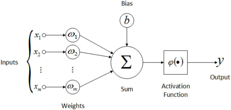
Mathematical model of the simulated neuron heavily inspired by the biological neuron:
Perceptrons were the original artificial neurons, with one layer of weights to learn and a binary threshold activation function. The weighted vote scheme effectively describes a hyperplane that divides the space of input vectors.
Learning with artificial neurons is about comparing output and reality and adjusting accordingly.
The non-linearity in the activation function keeps the whole network from collapsing into a linear operation. And non-linear systems are simply more capable and fun.
Learning weights
Credit Assignment Problem: If we layer neurons, how do we know which hidden layer node weights to nudge when learning?
Revenge of the knowledge engineers: Misky & Papert Perceptrons (1969), stalled research into connectionist ideas for a decade.
Maths breakthrough (well, statistical physics): Hopfield nets (1982)
From deterministic physical model to a probabilistic one: Boltzmann machines (1985)
Early brekathrough arrived when binary thresholding step was replaced with the softer function of phase transitions — the S-curve, the sigmoid. Moving from discrete output to continuous made a substantial qualitative difference. Sigmoids provided "a safe half-way house between dumb linear functions and hard step functions."
Backpropagation (1986): Assigning credit through a cascading process of nudges one layer at a time in a multi-layer perceptron configuration. (With differentiable, "soft" activation functions.)
Backpropagation is an efficient way to do gradient descent optimisation in a multilayer perceptron. No mathematical guarantee about avoiding local minima, but that's okay: high dimensionality helps, and we don't want to overfit with global optimum anyway.
Deep Learning
Backprop can handle one hidden layer, no problem. A few hidden layers, doable. A few more and it's not as smooth sailing.
Large neural networks are trickier to train, so the name of the game is designing networks that work well with the application in mind.
It's still backpropagation, today. Just with better optimisation, more data, faster computers. GPUs significantly speed up learning by enabling massively parallel computations.
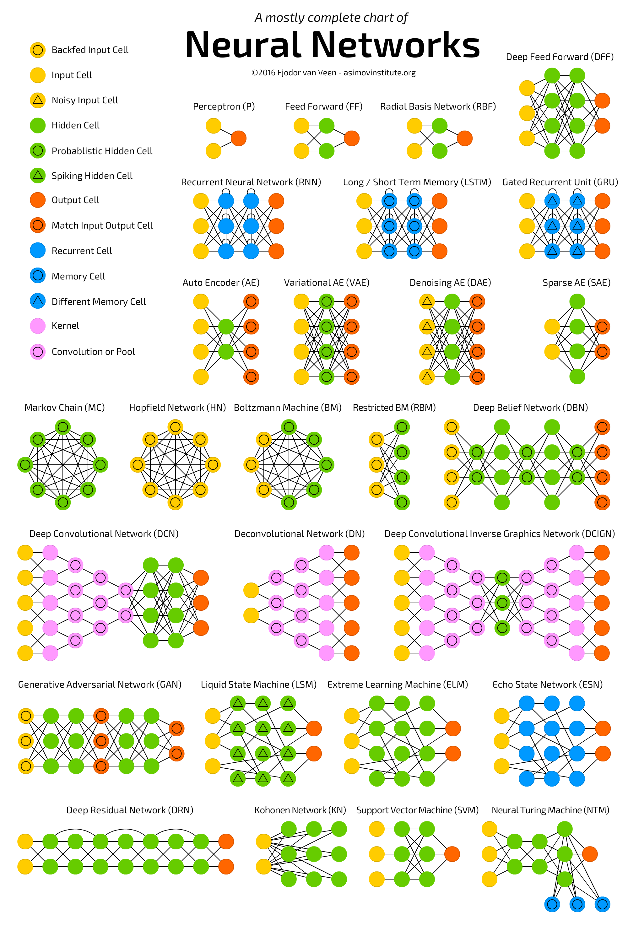
Some neural network architecture advances:
- Autoencoder (80s) — input and output are the same, network effectively learns a filter
- Recurrent Neural Network, RNN (80s, 90s) — network layers capture a temporal sequence
- Long short-term memory, LSTM (1997, 00s) — gate architecture RNN, with feedback loops
- Gated recurrent unit, GRU (2014) — simplified LSTM w/ forget gate
- Sparse Autoencoder (2010s) — large hidden layers, most of which are dark for any given input
- Stacking Autoencoders (2010s) — deeper layers use previous hidden layer as input/output
- Convolutional NNs (2010s, old idea) — deeper layers use previous output layer + some spatial coherence maths
- Generative adversarial network, GAN (2014) — two neural networks contest, optimising one another
- U-Net (2017) — deep convolutional net for image segmentation, with wires connecting early and late stages of the network
The Connectionists — Conclusion
Connectionists are in the business of reverse-engineering the brain, building computation inspired by the network structure of biological neurons. In artificial NNs, knowledge lives in network weights. Learning, inspired by Hebb's rule, is a matter of adjusting the weights.
A neural net can learn more complex functions, if it has many layers and nonlinear activations between the layers. Backpropagation was a key connectionist breakthrough that showied how to solve the credit assignment problem of a layered configuration.
Connectionists are currently the hottest tribe. Deep learning has been moving forward at a crazy pace. In recent years, research into various deep neural net architectures has produced a whole smörgåsbord of exciting results in a wide range of application areas.
The Evolutionaries
For Evolutionaries, learning is all about natural selection. By simulating it, we can build anything. The main challenge is learning structure: building the brain, building the nodes and connections that encode the solution to the problem. Parameter tuning can then follow as a secondary step.
The Evolutionary master algorithm is genetic programming, in which computer programs are mated and evolved like organisms in the natural world.
Nature's Algorithm
Ronald Fisher, early 20th C: Mathematical theory of evolution.
John Holland, 1960: A population of "genes" interacting, a disorderly search for fitness.
Fitness Function: Give a candidate program a numeric score to measure fitness for purpose.
Nature has no fitness function, but human systems naturally do.
System analogy of sexual reproduction:
- Gene — encoded data; a set of instructions, parameters for a process, a blueprint
- Population — a pool of genes, weighted to favour fit genes
- Crossover — exchange of data in which two parent genes split and recombine as offspring
- Mutation — point change in a data location in a gene
Artificial evolution allows for cheating, e.g., immortal genes.
Genetic Processing
Exploration-Exploitation Dilemma: If you've found something that kind of works, should you keep investing more in that, or should you try new things in hope of improvement?
Genetic algorithms have the capacity to make big jumps in the search. Not bound to a gradual, incremental process.
Schema theory: Each successful gene is a building block for future genes: the process is not wildly random, the combinatorial exponentials are working for you.
Benefit of crossover an open question. With just mutations and a large population, search reduces to hill-climbing, which a bit of randomisation can further stir.
Does sex optimise for mixability, and robustness against parasites?
Case: Fringeling
A real-world example, a little hobby project of mine using GeneticJS. Festival programming!
Main objective: Build a festival programme based on preferences. For a set of shows of interest (incl. showtimes), find a schedule/programme that maximises the number of shows seen over multi-day festival visit. Avoid overlap!
Secondary objective: Minimise travel time, minimise town crossings, leave 5-10min before buffers, leave time for lunch, etc.
Fringeling Gene:

Genetic Programming
John Koza, 1980s-: What if we could evolve not parameters, but the whole process?
Genetic Programming: Start with a population of random programs. Make use of crossover, mutation and survival to gradually evolve better programs until tests pass.
A computer program is really a tree of subroutine calls. Crossover at the subtree level turns one program into another. Correctness of a particular instance can be measured against known desired output. The challenge is to assemble the best sequence of subroutines and instructions.
Nature vs. Nurture
Connectionist take a simple structure and tune it, evolutionaries evolve structure. Evolving neural network structure?
Natural evolution is slow! Evaluating complex gene fitness is slow!
Culture is fast!
Baldwin effect: Learned behaviours become genetically hardwired.
(cf. Lamarckism: Transmission of acquired traits to offspring.)
"For the hardest problems [..] pure nature-inspired approaches are probably too uninformed to succeed, even given massive amounts of data. [..] We need to reason with larger chunks."
Hinton: Why carry around genetic information you can pick up with your senses?
The Evolutionaries — Conclusion
Evolutionaries believe that simulating evolution by natural selection is a nice compromise solution to the exploration-exploitation dilemma.
Genetic algorithms and programs excel in learning structure through the manipulation of "genes", encoded candidate solutions. From a gene population, the best solutions can be identified by a fitness function, a quality measure. Over many generations, the embedded building blocks of genes mutate and combine to form ever better solutions.
Genetic programming extends the evolutionary idea directly to programs, skipping parameter encoding. Even more expensive to evaluate and simulate, but more expressive. Baldwin effect and mixing with connectionist techniques may prove a fruitful direction.
Notes
-
No free lunch! Is it all just glorified hill-climbing?
-
Intuition from biology just superfluous? Compare with Hofstadter's fluid computation.
-
GP forgotten by the machine learning mainstream, but see how much mainstream ML is in GECCO today!
The Bayesians
For Bayesians, the main concern is uncertainty. All knowledge is uncertain, and learning itself is uncertain inference. The challenge is dealing with noisy, incomplete, and even contradictory information.
The Bayesian master algorithm is probabilistic inference through variations of Bayes' theorem, which tells us how to update our beliefs in light of new evidence.
Bayes' Theorem
P(A|B) = P(A) * P(B|A) / P(B)
A rule for updating your degree of belief in a hypothesis when you receive new evidence. If data agrees with hypothesis, hypothesis probability goes up, otherwise down. The challenge is in learning efficiently from a whole set of data, for a whole set of hypotheses.
For Bayesians, learning is about model selection based on data.
Principle of indifference: In the absence of any relevant evidence, belief in all outcomes under consideration should be distributed equally. (Epistemic probability)
Prior probability: (Subjective, intuitive) probability of an event, before seeing any evidence.
Posterior probability: Probability after evidence has been weighed.
Conditional probability: Probability of an event, given another event. P(A|B) : probability of event A, given event B has occurred.
Bayes' formula is fairly straightforward, the tricky part is coming up with the probabilities, and doing the computation.
For frequentists, only valid way of deriving probabilities is through statistics. Bayesians are happy with subjective estimates, and are more comfortable with assigning probabilities to one-off events.
Deriving the theorem
- "The more likely the effect, given the cause, the more likely the cause given the effect."
▲ P(effect|cause) ⇒ ▲ P(cause|effect)
- Common effects make particular causes less likely.
▲ P(effect) ⇒ ▼ P(cause|effect)
- More likely a cause a priori, more likely the cause a posteriori — all else equal.
▲ P(cause) ⇒ ▲ P(cause|effect)
- And so:
P(cause|effect) = P(cause) * P(effect|cause) / P(effect)
Lego Example
Counting in two ways is a powerful proof tool in mathematics.
Bayes' theorem can be shuffled to be symmetrical:
P(cause|effect) * P(effect) = P(effect|cause) * P(cause)
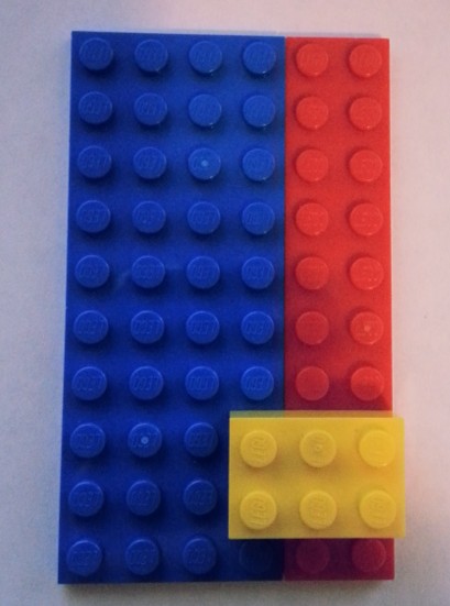
- 6x10 = 60 Pegs
- 4x10 = 40 Blue Pegs
- 2x10 = 20 Red Pegs
- 3x2 = 6 Yellow Pegs
- P(Blue) = 40/60 = 2/3
- P(Red) = 20/60 = 1/3
- P(Yellow) = 6/60 = 1/10
- P(Blue) + P(Red) = 1
- P(Blue) + P(Red) + P(Yellow) = no go
- P(Yellow | Red) = 4/20
- P(Red | Yellow) = 4/6
- P(Yellow|Red)*P(Red) = 4/20 * 20/60 = 4/60
- P(Red|Yellow)*P(Yellow) = 4/6 * 6/60 = 4/60
Naïve Bayes
For complex effects, with many contributing causes, it is necessary to fight combinatorial explosion with simplifying assumptions.
George Box, frequently: "All models are wrong, but some are useful."
Naïve Bayes: All effects are independent, given cause.
P(fever & cough | flu) = P(fever | cough, flu) * P(cough | flu) P(fever & cough | flu) = P(cough | fever, flu) * P(fever | flu)
[naïve assumption]
P(fever & cough | flu) = P(fever | flu) * P(cough | flu)
Having a fever doesn't change the probability of having a cough, if you have the flu.
OR: If you have the flu, knowing that you have a fever gives no new information.
(Fever and cough are NOT independent in general.)
Naïve Bayes classifiers are very popular, and quite powerful. "Just a matter of counting how many times each attribute occurs with each class."
Naïve Bayes is closely related with perceptrons! The percepton adds weights, while Naïve Bayes multiplies probabilities — if you take a logarithm, multiplication becomes addition.
Naïve Bayes captures pairwise correlations between inputs and outputs, which is often plenty, but there are of course more complex patterns to learn.
Markov Models
Next step after total independence, the bare minimum of structure.
Markov Property (loosely): For a sequence, assume that the probability of the next one depends on the previous one (only).
[with some notation abuse] P(xn | xn-1 ← xn-2 ← ... ← x0) = P(xn | xn-1)
A Markov chain is a discrete Markov process that moves from state to state. There exists a vast mathematical literature on Markov processes.
Hidden Markov Model (HMM): A Markov process of observations, plus an unobservable, hidden state that is dragged along.
HMM example, speech recognition:
Task: Infer word from sound
Hidden states: written words
Observations: sounds spoken
Model 1: P(wordn | wordn-1), where wordi is a hidden state
Model 2: P(soundn | wordn)
Kalman filter: Roughly a HMM with continuous variables instead of discrete states.
Bayesian Networks
Judea Pearl, early 1980s: It's OK to have a complex network of dependencies among random variables, provided each variable depends directly on only a few others.
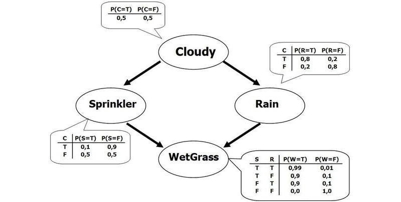
Byesian Network (BN): Complex probability configurations can be represented as a graph (without cycles) plus a probability table per variable of its parents.
BNs enable dramatic simplification of the mathematics: the full set of probabilities can be encoded into fewer probability values. This is made possible by conditional independence.
The probability of a complete state is the product of the corresponding paths through the graph. Even possible to compute probabilities for states never observed. A Bayesian network tells a story.
Bayesian networks are the lingua franca for encoding probability configurations: Naïve Bayes, Markov models, HMMs can all be modelled as Bayesian networks.
Bayesian inference is frequently doable without exponential blowup, but not always. Sometimes large BNs have nodes with too many parents, and simpler OR-distributions need to be learned instead — details can be blurred or abstracted away as an assumption. Collapsing paths into megavariables helps only so far.
More powerful techniques needed for complex Bayesian network configurations, with loops an all:
- Loopy belief propagation: pretend the graph has no loops, and pass probabilities back and forth until convergence (not guaranteed to succeed, but works in the real world)
- Markov chain Monte Carlo (MCMC): do a random walk, jumping from network state to state in such a way that in the long run, each state is visited in proportion to its probability
MCMC is effectively a numerical approximation. Instead of doing inference on an explicit BN, design a Markov chain that converges (via MCMC) to the distribution of the target BN. We can then answer inference questions about the BN by drawing samples from the MCMC.
MCMC is in heavy use today. Not just for probability configurations, but for integrating all kinds of functions, in particular those that don't have a clean analytical solution. Unfortunately MCMC can be very slow to converge, and has a habit of fooling the observer: real-world probabilities are sharp.
A vast literature exists on MCMCs and all kinds of applications of Bayesian inference.
Bayesian learning
For Bayesians, learning is just another kind of inference:
P(hypothesis|data) = P(hypothesis) * P(data|hypothesis) / P(data)
Maximum Likelihood Principle: Of all the hypotheses available, pick the one in which seeing the data is most likely.
Likelihood of a hypothesis is P(data|hypothesis), so select the hypothesis that maximises the value. But Bayesians are never sure: instead of selecting a hypothesis, compute posteriors for all hypotheses. Entertain all hypotheses when making predictions.
There is no truth: it's all just a prior distribution over hypotheses that becomes the posterior distribution after data has been seen. Expensive to compute, which is why we crank MCMC. In real-world situations, most hypotheses have a tiny posterior probability and can safely be ignored. Most probable hypothesis alone is usually a reasonable approximation. Having more data helps concentrate the distribution.
Bayesians can go with a default prior and reduce to maximum likelihood, but can also use the prior distribution to encode domain knowledge — the data will override prior mistakes.
For a Bayesian, probability is a subjective degree of belief, so educated guesses are OK: inference calculus keeps all guesses consistent.
False independence assumption comes back to bite you in high-end models. The strength of Naïve Bayes is how simple it is to process.
Markov Networks: A graph of undirected arcs; a set of features and weights that define a probability distribution. Two variables are connected, if they feature together in some variable.
Bayesians vs. Symbolists
Bayesian CONs:
- Expensive inference
- Have to deal with all these prios and other numbers
- Hypothesis bookkeeping overhead
- No composing knowledge on the fly
- Inventing a probability distribution over data stores tricky
- Logic encodes anything, Bayesians limited to direct causality
- No relations: Bayesians stuck learning one truth table
Bayesian PROs:
- Logic is brittle, exceptions never end
- Logic cannot handle ambiguity, noise, or conflicting data
- Logic cannot trust learned knowledge: falsehood ⇒ anything
Unifying logic and probability is challenging. Domingos believes in Markov Logic Networks.
Case: Gen
Gen is a new probabilistic computing toolset built on top of Julia-lang.
Describe your probablistic inference task as a simulation of sorts. Framework does the heavy lifting (cf. autograd in PyTorch, etc.).
"Gen is a new probabilistic programming platform that aims to make it possible to do real-time inference in generative models by combining of model-based search, data-driven neural network inference, and state-of-the-art Monte Carlo techniques. Gen is thus a multi-paradigm platform for probabilistic artificial intelligence research that aims to be efficient and expressive enough for general-purpose use."
Presentation @ Strange Loop 2019
The Bayesians — Conclusion
For Bayesians, all knowledge is uncertain, and learning is a form of probabilistic inference.
Bayes Theorem tells us how to do inference, how to update beliefs in light of new evidence. The challenge is in generating the probabilities and doing the inference computation in complex configurations.
Naïve Bayes makes the assumption that all effects are independent, given cause. This captures the often critical pairwise correlations while remaining straightforward to compute.
Various Markov models improve fidelity by allowing for more structure, at a computational cost. Markov processes make a "forgetful" assumption about history: in a sequence, only the previous step can influence the next state.
Bayesian Networks capture complexities of probabilistic configurations in a convenient graphical model that tells a story. Markov chain Monte Carlo (MCMC) is a powerful technique for sampling complex probability distributions and other functions.
Bayesian learning is an approach to data-driven hypothesis selection, in which a range of probable hypotheses are pushed through the inference process.
P(hypothesis|data) ∝ P(hypothesis) * P(data|hypothesis)
The Analogizers
For Analogizers, learning is about recognising similarities between situations and inferring novel similarities. The challenge is determining how similar two things are.
Similarity is one of the central ideas of machine learning, and analogizers in all their guises are its keepers. According to Domingos, the analogizer's master algorithm is the support vector machine, which "figures out which experiences to remember and how to combine them to make new predictions."
Note: The Analogizer tribe is the least cohesive of the five. Personally, I don't believe SVMs capture the essence of analogy-making in the Hofstadterian sense.
Nearest-neighbour algorithm
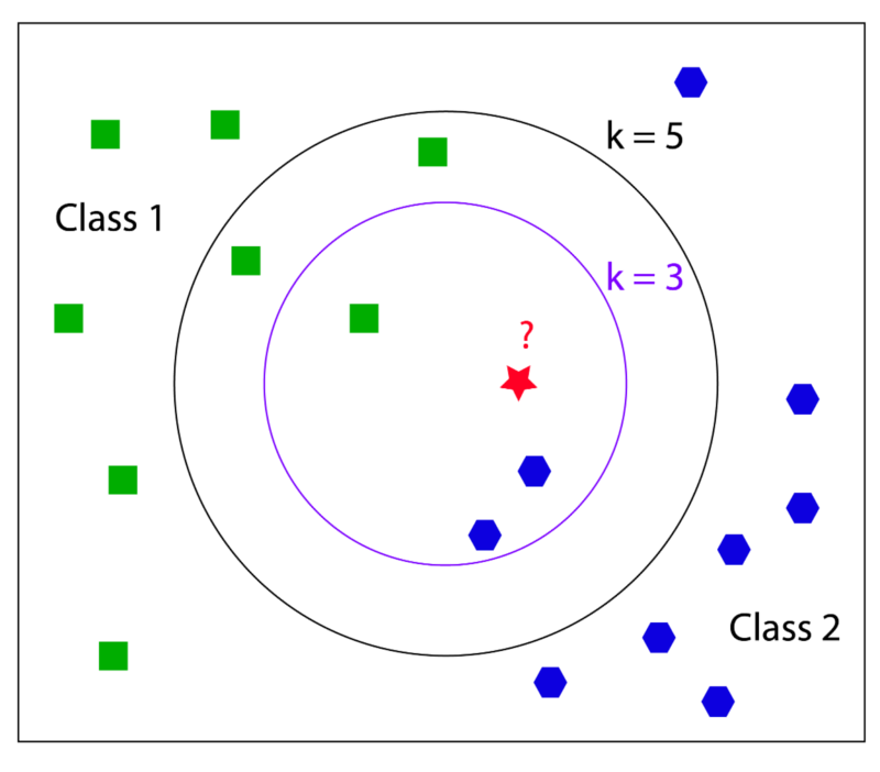
Collect data without processing, and at test time find the item nearest to the new item. If that one meets the spec, so does the new one. Parameter k determines the number of similar items to use in determining type.
K-NN forms a lazy, local model of the data and at query time resolves the classification boundaries around the target item. In a sense, each data point is a mini classifier, predicting the class of all queries.
Nearest-neighbour algorithm (k=1) is noisy and overfitting, but by adding a few extra nodes the aggregate vote becomes more robust. Cost is fidelity: more voting items "blurs" the classification boundary, with detail being lost. (K goes up, variance goes down, bias goes up.)
It is also possible to weight the voting neighbours: votes don't count equally, being closer gives you a louder voice.
Collaborative Filtering: People who agree in the past are likely to agree in the future. People's preferences have regularity across the population. Or, "people have types".
Recommender systems are a big business. (See also filter bubble.)
Nearest-neighbour systems can be made more performant by removing samples correctly classified by their neighbours.
Nearest-neighbour was the first algorithm that could take advantage of unlimited amounts of data and learn arbitarily complex concepts.
Trouble in high dimensions
Curse of dimensionality: A range of issues that arise when processing data in high-dimensions spaces that do not occur in low-dimensional settings. (High being thousands or more, low being, say, 2D or 3D.)
Nearest-neighbour is in trouble in high-dimensional settings: all dimensions contribute to similarity measure, but most of them are irrelevant for the application at hand. With enough attributes, the small contributions of meaningless similarities swamp out the similarity in the attributes of interest.
There's also more to learn in higher dimensions, more data needed for robust classification.
Even more alarmingly, the notion of similarity breaks down in high dimensions, our intuitions no longer hold. "The hyper-orange is all skin, you'll never be done peeling it!"
Even the trusty normal distribution fails on us, with samples near the mean being less probable than those further away. Randomly distributed points in hyperspace are closer to the sides of the hypercube than to one another.
Fighting the curse begins by getting rid of irrelevant dimensions. Information gain can be used as a measure, as is done with decision trees. Meta-learners can help identify the attributes that matter. Another option is to add weights to the attributes.
Blessing of non-uniformity: Data lives in high dimensions, but is not uniformly spread out in hyperspace. A tiny fraction of all possible data points are reasonable, and the reasonable ones "all live together in a cozy little corner of hyperspace".
Support Vector Machines
Vladimir Vapnik, 1990s: Weighted k-NN on steroids, but not all borders are created equal.
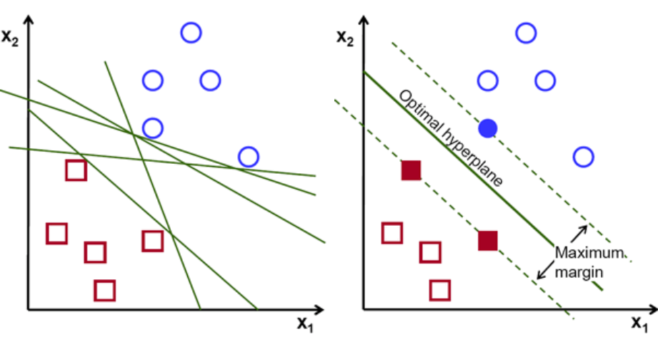
In a Support Vector Machine (SVM), the classifier frontier is determined by a set of examples and their weights, together with a similarity measure. Weighted average determines the class. SVMs maximise the margin of the classification boundary. This maximisation makes SVMs quite resistant to overfitting.
SVMs remember only the key examples required to pin down the frontier. SVMs can learn smooth frontiers, but need to be constrained, or the learning mechanism becomes unstable. The support vectors are active constraints during leaning. Contraint violations are possible — to counteract noise — but discouraged through penalties.
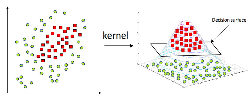
Kernel Trick: SVMs always create straight planes in the hyperspace, no matter how curvy the frontier may appear. SVMs operate by finding a maximum-margin hyperplane in the kernel space to which data is mapped from the original domain by a kernel function.
SVMs can be seen as a generalisation of perceptron, because a hyperplane boundary between classes is what you get when you use a particular simliarity measure. SVMs are kind of like a hidden layer with the weighted averages serving as the output layer.
With deep learning, connectionists have regained the upper hand: SVMs always have just one layer, whereas networks with many layers can express many functions more compactly.
Essence of Analogy
Similarity is a spectral quality. There are simple ways of being similar, and more complicated ones. We can apply analogical reasoning to all kinds of objects, not just vectors of attributes.
Two things are similar if they agree in some aspects. And if they agree in some aspects, they probably agree on some other aspects. This is the essence of analogy.
The challenge of analogical reasoning is to figure out how similar two things are and then deciding what else to infer from their similarities. It's a matter of finding relevant information from the available data.
Analogy is most powerful when crossing problem domain boundaries. Humans do this kind of structural mapping all the time. Some have attempted to build algorithms around this notion, but with very limited success.
A.H.: Hofstadter et al. give a pretty solid trashing of Gentner and others and their outrageous claims of having built functional structural mapping algorithms.
Douglas Hofstadter's entire research career revolves around analogy-making. Output from this work includes the acclaimed "Gödel, Escher, Bach: An Eternal Golden Braid".
The Analogizers — Conclusion
Similarity is a central idea in machine learning, manifesting as a family of functions ranging from simple similarity to complex analogies. The Analogizer tribe is the least cohesive of the five.
In nearest-neighbour classification, a lazy, local model of the data is queried with new items. Through a simple similarity measure, a vote over nearby items, nearest-neighbour classifiers can establish boundaries in arbitrarily complex concept space. One can add weights to nearest-neighbour for a biased vote.
Curse of high-dimensionality, the peculiar deformations of high-dimensional hyperspace that trip up our intuition and our algorithms, is a major challenge in machine learning. Fortunately our data is typically non-uniform and we can identify locals pockets of hyperspace in which our methods work fine.
Support Vector Machines maximise the margin around a classification boundary. The support vectors that straddle the margin, the voting weights, and data mapping kernels together configure a hyperspace in which the SVM finds a straight hyperplane that best divides the data.
Higher abstraction similarities lead to analogy-making, where the main challenge is choosing useful representations and identifying relevant information. Some claim analogy is the essence of cognition.
The Big Picture
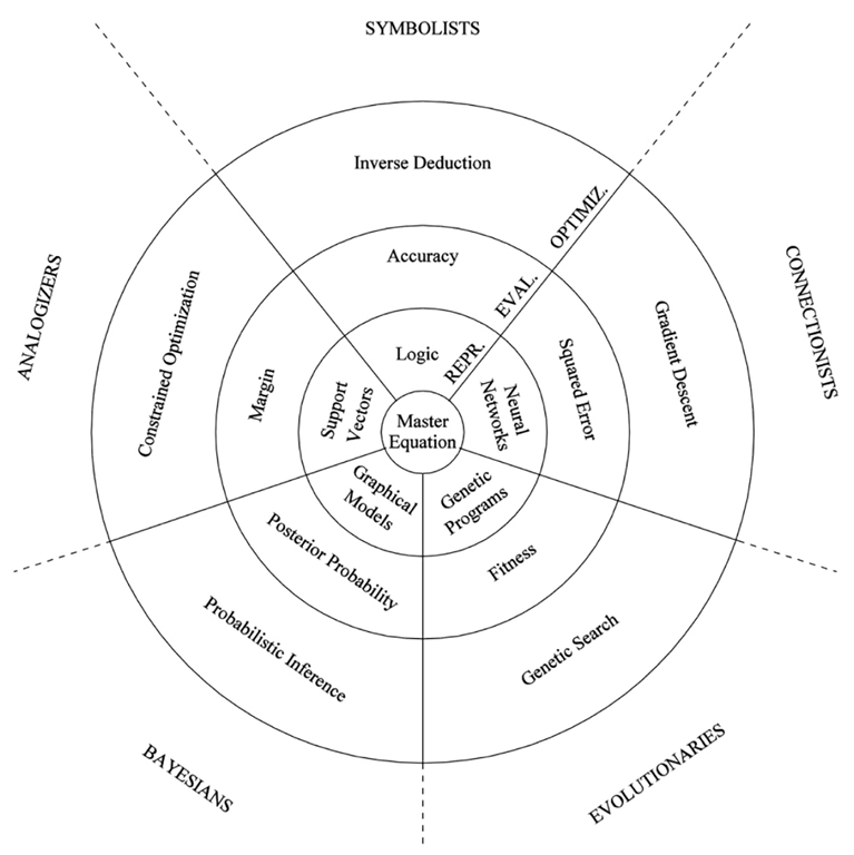 Source, Domingos — Master Algorithm
EXTRA: Self-Learning (The Sixth Tribe)
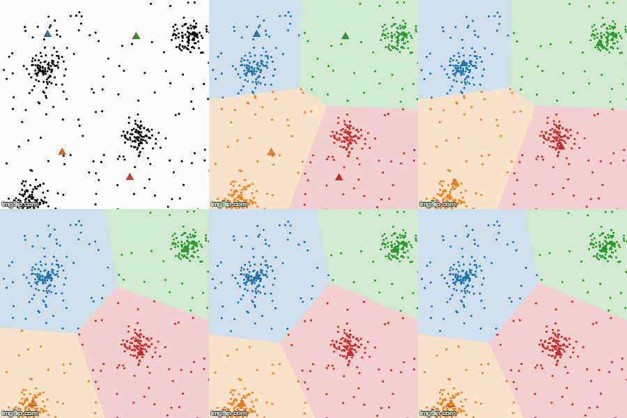
k-Means
Data clustering without human guidance.
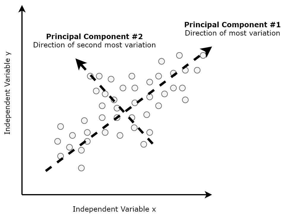
Principal Component Analysis (PCA)
Discovering the primary dimensions of data.
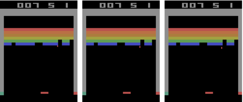
Reinforcement Learning
Teaching agents to take actions in an environment through autonomous exploration and exploitation.
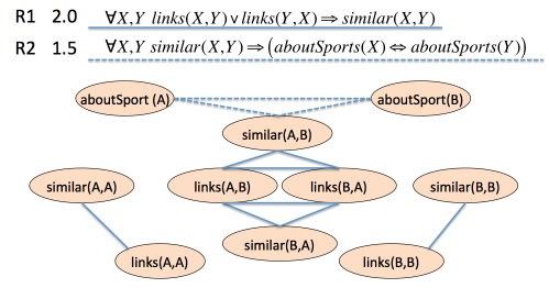
Relational Learning
Modelling uncertainty and representing knowledge in a complex relational structure.
